GBDT
In Gradient Boosting, classification is performed by sequential accumulation of real-valued scores. The implementation follows scikit-learn’s One-vs-Rest (OVR) scheme: for a problem with \(|C|\) classes, there are \(|C|\) independent score channels.
HCPN Formalization
The GBDT model is represented as a 3-level HCPN:
Modules \(S_{GBDT} = \{s_{GBDT}, \; s_{channel}, \; s_{DT}\}\):
\(s_{GBDT}\) — the top-level module with class-channel substitution transitions and the activation transition.
\(s_{channel}\) — the mid-level module representing a single class channel’s sequential boosting loop.
\(s_{DT}\) — the leaf module (see Decision Tree), reused \(|C| \times K\) times (once per boosting stage per class).
Top-Level Module \(s_{GBDT}\)
with:
\(P = \{P_{in}, \; {P_{score}}^{(1)}, \dots, {P_{score}}^{(|C|)}, \; P_{out}\}\).
\(C(P_{in}) = \text{VEC}\), \(C({P_{score}}^{(c)}) = \text{SCORE}\), \(C(P_{out}) = \text{LABEL}\).
\(T = \{{t_{ch}}^{(1)}, \dots, {t_{ch}}^{(|C|)}, \; t_{act}\}\) — \(|C|\) substitution transitions (one per class channel) plus one regular activation transition.
Submodule function:
Port-socket bindings for each \({t_{ch}}^{(c)}\):
\(P_{in}\) (In port of \(s_{channel}\)) \(\leftrightarrow\) \(P_{in}\) (socket in \(s_{GBDT}\)).
\(P_{result}\) (Out port of \(s_{channel}\)) \(\leftrightarrow\) \({P_{score}}^{(c)}\) (socket in \(s_{GBDT}\)).
Mid-Level Module \(s_{channel}\) (Boosting Loop)
Each class channel is a module that sequentially accumulates contributions from \(K\) boosting stages:
with:
\(P = \{P_{in}, \; P_{accum}, \; P_{stage}, \; P_{result}\}\).
\(C(P_{in}) = \text{VEC}\), \(C(P_{accum}) = \text{SCORE}\), \(C(P_{stage}) = \text{STAGE}\), \(C(P_{result}) = \text{SCORE}\).
\(PT(P_{in}) = In\), \(PT(P_{result}) = Out\).
\(T = \{{t_{stage}}^{(1)}, \dots, {t_{stage}}^{(K)}, \; t_{finalize}\}\) — \(K\) substitution transitions (one per boosting stage) plus a finalize transition.
Initial marking:
\(I(P_{accum}) = \{s_0\}\) — the initial score (bias) derived from scikit-learn’s prior estimator (
DummyClassifier):
\(I(P_{stage}) = \{1\}\) — stage counter starts at 1.
Submodule function:
Each substitution transition \({t_{stage}}^{(k)}\) is refined into a DT leaf module containing the rules of the \(k\)-th boosting tree for this class channel.
Port-socket bindings for each \({t_{stage}}^{(k)}\):
\(P_{in}\) (In port of \(s_{DT}\)) \(\leftrightarrow\) \(P_{in}\) (socket in \(s_{channel}\)).
\(P_{out}\) (Out port of \(s_{DT}\)) \(\leftrightarrow\) \(P_{accum}\) (socket in \(s_{channel}\)).
Sequential accumulation logic:
The stage counter \(\kappa \in P_{stage}\) enforces sequential firing. For each stage \(k\):
Guard on \({t_{stage}}^{(k)}\): \([\kappa = k]\) — the substitution transition is only enabled at the correct stage.
After the DT sub-module fires (exactly one rule matches, producing \(\eta \cdot {v_k}^{(c)}\)), the channel module’s arc expressions update:
\(P_{accum} \leftarrow s + \eta \cdot {v_k}^{(c)}\) (accumulated score).
\(P_{stage} \leftarrow \kappa + 1\) (advance counter).
Finalize transition \(t_{finalize}\):
Guarded by \([\kappa = K{+}1]\), this regular transition consumes the final accumulated score from \(P_{accum}\) and deposits it in the output port \(P_{result}\).
Note
Within each boosting stage, the DT sub-module’s internal mutual exclusivity guarantees that exactly one leaf fires. The stage counter ensures strict sequential ordering across stages, so at most one substitution transition is enabled at any time.
Activation Transition \(t_{act}\)
After all \(|C|\) channel modules complete (each depositing a terminal score in \({P_{score}}^{(c)}\)), the activation transition \(t_{act}\) in the top-level module \(s_{GBDT}\) fires. It is a synchronization transition with \(|C|\) input arcs — one from each \({P_{score}}^{(c)}\) — collecting the terminal scores \({s_K}^{(1)}, {s_K}^{(2)}, \dots, {s_K}^{(|C|)}\) in a single atomic step. The activation is a two-step process:
Probability computation:
Decision:
Note
In the multiclass case, because softmax is a monotonic transformation, \(\arg\max\) can be applied directly to the raw scores \({s_K}^{(c)}\) without computing the softmax probabilities, which is what the implementation does.
Fusion set \(FS_{GBDT}\):
The input place \(P_{in}\) is fused across the top module, all channel sub-modules, and all DT sub-module instances. Every tree in every channel evaluates the same input vector \(x\).
Summary of the OVR score accumulation:
where \(K\) is the number of boosting stages, \(\eta\) is the learning rate, and \({v_k}^{(c)}\) is the leaf value of the matched rule in tree \(k\) for class \(c\).
The figure below depicts the additive composition for a single class channel. The place \(P_{initial\_score}\) holds the bias token \(s_0\). Inside the additive boosting cycle, each gradient step transition \(T_{tree\_k}\) adds \(\eta \cdot v_k\) to the accumulator. After the final iteration, the activation transition \(T_{activation}\) (sigmoid or softmax) converts the raw score into a class probability and deposits the result in \(P_{final\_prediction}\). For multiclass problems, \(|C|\) such channels operate in parallel, and the activation transition collects all channel scores before producing the final label.
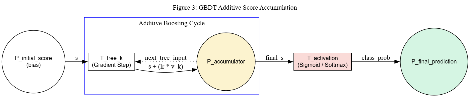
HCPN for GBDT (single class channel view): initial bias score, sequential accumulation via substitution transitions (each refining to a DT module), and a final activation transition (sigmoid/softmax).
Numerical Induction Example
The following example demonstrates that the HCPN construction correctly accumulates scores for a channel with \(K\) boosting stages and remains valid when extended to \(K+1\) stages. A binary classification problem is used for clarity (single channel, sigmoid activation).
Setup: Feature space \((x_1, x_2)\), classes \(\{0, 1\}\), learning rate \(\eta = 0.1\). Training set has 60% positive samples, so the initial score is:
Base case \((K = 2)\):
Two boosting stages, each with a small decision tree:
Stage |
Rule |
Guard |
Leaf value \(v\) |
|---|---|---|---|
\(k = 1\) |
\(r_{1a}\) |
\(x_1 \leq 3.0\) |
\(+2.4\) |
\(k = 1\) |
\(r_{1b}\) |
\(x_1 > 3.0\) |
\(-1.8\) |
\(k = 2\) |
\(r_{2a}\) |
\(x_2 \leq 5.0\) |
\(+1.5\) |
\(k = 2\) |
\(r_{2b}\) |
\(x_2 > 5.0\) |
\(-0.9\) |
HCPN state trace for input \(x = (2.0, \; 7.0)\):
Initial state: \(P_{accum} = 0.4055\), \(P_{stage} = 1\).
Stage 1 (\(\kappa = 1\)):
Guard \([\kappa = 1]\) is true, so \({t_{stage}}^{(1)}\) is enabled.
DT sub-module fires: \(G(r_{1a}) = [2.0 \leq 3.0] = \text{true}\), matched leaf value \(v_1 = +2.4\).
\(P_{accum} \leftarrow 0.4055 + 0.1 \times 2.4 = 0.4055 + 0.24 = 0.6455\).
\(P_{stage} \leftarrow 2\).
Stage 2 (\(\kappa = 2\)):
Guard \([\kappa = 2]\) is true, so \({t_{stage}}^{(2)}\) is enabled.
DT sub-module fires: \(G(r_{2b}) = [7.0 > 5.0] = \text{true}\), matched leaf value \(v_2 = -0.9\).
\(P_{accum} \leftarrow 0.6455 + 0.1 \times (-0.9) = 0.6455 - 0.09 = 0.5555\).
\(P_{stage} \leftarrow 3\).
Finalize (\(\kappa = 3 = K{+}1\)):
\(t_{finalize}\) fires, deposits \(s_2 = 0.5555\) in \(P_{result}\).
Activation:
Accumulated score matches the formula:
Inductive step \((K = 2 \to K + 1 = 3)\):
A third boosting stage is added with a new decision tree:
Stage |
Rule |
Guard |
Leaf value \(v\) |
|---|---|---|---|
\(k = 3\) |
\(r_{3a}\) |
\(x_1 \leq 4.0 \;\wedge\; x_2 > 6.0\) |
\(+1.2\) |
\(k = 3\) |
\(r_{3b}\) |
\(x_1 \leq 4.0 \;\wedge\; x_2 \leq 6.0\) |
\(-0.5\) |
\(k = 3\) |
\(r_{3c}\) |
\(x_1 > 4.0\) |
\(-1.0\) |
The HCPN is extended by:
Adding a substitution transition \({t_{stage}}^{(3)}\) to \(T_{sub}\) in \(s_{channel}\).
Mapping \(SM_{ch}({t_{stage}}^{(3)}) = s_{DT}\).
Port-socket bindings identical to existing stages.
Updating \(t_{finalize}\)’s guard from \([\kappa = 3]\) to \([\kappa = 4]\).
Updating \(\text{STAGE}\) colour set from \(\{1,2,3\}\) to \(\{1,2,3,4\}\).
HCPN state trace for input \(x = (2.0, \; 7.0)\) (continued from \(K = 2\) ):
After stages 1 and 2, the state is identical: \(P_{accum} = 0.5555\), \(P_{stage} = 3\). The new stage 3 fires:
Stage 3 (\(\kappa = 3\)):
Guard \([\kappa = 3]\) is true, so \({t_{stage}}^{(3)}\) is enabled.
DT sub-module fires: \(G(r_{3a}) = [2.0 \leq 4.0] \wedge [7.0 > 6.0] = \text{true}\), matched leaf value \(v_3 = +1.2\).
\(P_{accum} \leftarrow 0.5555 + 0.1 \times 1.2 = 0.5555 + 0.12 = 0.6755\).
\(P_{stage} \leftarrow 4\).
Finalize (\(\kappa = 4 = K{+}1\)):
\(t_{finalize}\) fires, deposits \(s_3 = 0.6755\) in \(P_{result}\).
Activation:
Accumulated score matches the extended formula:
Why the invariant is preserved: Adding stage \(K+1\) to a valid \(K\)-stage channel requires only:
One new substitution transition \({t_{stage}}^{(K+1)}\) with guard \([\kappa = K{+}1]\).
\(SM_{ch}({t_{stage}}^{(K+1)}) = s_{DT}\) — same leaf module type, new rule set.
Port-socket bindings identical to all existing stages.
Update \(t_{finalize}\)’s guard from \([\kappa = K{+}1]\) to \([\kappa = K{+}2]\).
The stage counter ensures that stages 1 through \(K\) execute identically to the \(K\)-stage case (their guards and rule sets are unchanged). Stage \(K+1\) fires only after \(P_{stage} = K{+}1\), extending the accumulation by exactly \(\eta \cdot v_{K+1}\):
The finalize transition then deposits the updated score. The DT invariant guarantees exactly one rule fires per stage, the stage counter guarantees sequential order, and the additive formula generalises directly.
Conclusion: By induction on \(K\), the GBDT HCPN construction correctly accumulates scores for any number of boosting stages. Each additional stage adds one substitution transition and one additive contribution, without affecting the existing stages or their determinism guarantees.