Random Forest
The HCPN framework enables a natural representation of the Random Forest: each individual tree is an instance of the leaf module \(s_{DT}\), composed into a top-level module via substitution transitions, port-socket bindings, and fusion places.
HCPN Formalization
For a Random Forest with \(N\) trees, the HCPN is:
Modules \(S_{RF} = \{s_{RF}, \; s_{DT}\}\):
\(s_{RF}\) — the top-level module containing the voting logic.
\(s_{DT}\) — the leaf module (see Decision Tree), reused \(N\) times.
Top-level module \(s_{RF}\):
with:
\(P = \{P_{in}, P_{collect}, P_{out}\}\) — input, collector, and output places.
\(C(P_{in}) = \text{VEC}\), \(C(P_{collect}) = \text{PROB}\), \(C(P_{out}) = \text{LABEL}\).
\(T = \{t_{tree_1}, \dots, t_{tree_N}, \; t_{vote}\}\) — \(N\) substitution transitions plus one regular aggregation transition.
\(t_{vote}\) — a regular transition (not in \(T_{sub}\)) that performs soft voting.
Submodule function \(SM_{RF}\):
Each substitution transition \(t_{tree_k}\) is refined into the DT leaf module. Although the same module definition \(s_{DT}\) is referenced \(N\) times, each instance carries its own rule set (extracted from the \(k\)-th tree in the forest).
Port-socket bindings \(PS_{RF}\):
For each substitution transition \(t_{tree_k}\):
The In port \(P_{in}\) of \(s_{DT}\) is bound to socket \(P_{in}\) in \(s_{RF}\).
The Out port \(P_{out}\) of \(s_{DT}\) is bound to socket \(P_{collect}\) in \(s_{RF}\).
Colour compatibility is ensured: the DT module’s output port produces \(\text{PROB}\) vectors (the normalised class distribution at the matched leaf), matching \(C(P_{collect}) = \text{PROB}\).
Note
In the RF context, the DT module’s output arc expression is adapted: instead of depositing a discrete label, it yields the normalised class distribution \(\mathbf{p}_k \in [0,1]^{|C|}\) at the matched leaf. The port colour is therefore \(\text{PROB}\) rather than \(\text{LABEL}\).
Fusion set \(FS_{RF}\):
The input place \(P_{in}\) is a fusion place shared across the top module and all \(N\) DT sub-module instances. Every tree evaluates the same input token \(x\) without duplicating it.
Soft Voting (transition \(t_{vote}\) ):
The aggregation transition \(t_{vote}\) consumes all \(N\) probability tokens from \(P_{collect}\) (enabled only when \(|P_{collect}| \geq N\)). Its output arc expression computes:
This matches the default behaviour of scikit-learn’s RandomForestClassifier, which uses soft voting via predict_proba averaging.
The following figure shows the parallel composition. Each sub-page \(Tree_k\) is an independent CPN module whose output probability vector is collected in \(P_{collector}\). The aggregation transition \(T_{voter}\) computes the averaged probabilities and deposits the winning class in \(P_{final\_class}\).
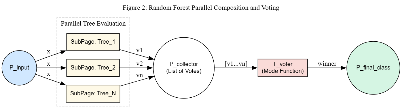
HCPN for Random Forest: \(N\) substitution transitions (each refining to a DT module) feed probability vectors into a collector place, followed by a soft-voting aggregation transition.
Note
The figure labels the aggregation transition as “Mode Function” for visual simplicity. In the actual implementation, soft voting (probability averaging) is used as the primary path; hard voting (mode) exists only as a fallback when class distribution data is unavailable.
Numerical Induction Example
The following example demonstrates that the HCPN construction preserves correct soft-voting semantics for a forest with \(N\) trees and remains valid when extended to \(N+1\) trees.
Setup: Binary classification with classes \(\{0, 1\}\). Input \(x = (3.0, \; 7.0)\).
Base case \((N = 2)\):
Two decision trees, each producing a probability vector at its matched leaf:
Tree |
Matched rule guard |
Output \(\mathbf{p}_k\) |
|---|---|---|
\(T_1\) |
\(x_1 \leq 5.0\) (true) |
\((0.8, \; 0.2)\) |
\(T_2\) |
\(x_2 > 4.0\) (true) |
\((0.6, \; 0.4)\) |
HCPN state trace:
\(P_{in}\) holds token \(x = (3.0, 7.0)\). Fusion set shares it with both DT sub-modules.
\(t_{tree_1}\) fires (substitution transition refines to \(s_{DT}^{(1)}\)): one rule matches, deposits \((0.8, 0.2)\) in \(P_{collect}\).
\(t_{tree_2}\) fires (substitution transition refines to \(s_{DT}^{(2)}\)): one rule matches, deposits \((0.6, 0.4)\) in \(P_{collect}\).
\(P_{collect}\) now contains 2 tokens. \(t_{vote}\) is enabled (requires \(N = 2\) tokens):
Result: class \(0\). \(\checkmark\)
Inductive step \((N = 2 \to N + 1 = 3)\):
A third tree \(T_3\) is added to the forest. The HCPN is extended by:
Adding a substitution transition \(t_{tree_3}\) to \(T_{sub}\) in the top module.
Mapping \(SM_{RF}(t_{tree_3}) = s_{DT}\).
Binding its ports: \(P_{in} \leftrightarrow P_{in}\) (via fusion), \(P_{out} \leftrightarrow P_{collect}\).
Updating \(t_{vote}\)’s enabling condition to require \(N+1 = 3\) tokens.
Tree |
Matched rule guard |
Output \(\mathbf{p}_k\) |
|---|---|---|
\(T_1\) |
\(x_1 \leq 5.0\) (true) |
\((0.8, \; 0.2)\) |
\(T_2\) |
\(x_2 > 4.0\) (true) |
\((0.6, \; 0.4)\) |
\(T_3\) |
\(x_1 \leq 5.0 \;\wedge\; x_2 > 6.0\) (true) |
\((0.3, \; 0.7)\) |
HCPN state trace:
\(P_{in}\) holds \(x\). Fusion shares it with all 3 sub-modules.
Three substitution transitions fire independently. \(P_{collect}\) receives 3 tokens.
\(t_{vote}\) is enabled (requires \(N+1 = 3\) tokens):
Result: class \(0\). \(\checkmark\)
Why the invariant is preserved: Adding a tree \(T_{N+1}\) to a valid \(N\)-tree HCPN requires only:
One new substitution transition \(t_{tree_{N+1}}\) with \(SM(t_{tree_{N+1}}) = s_{DT}\).
Port-socket bindings identical to those of all existing trees.
The fusion set \(FS\) is unchanged — \(P_{in}\) is already shared.
The voting transition \(t_{vote}\) updates its arc weight from \(N\) to \(N+1\).
The DT leaf module guarantees exactly one rule fires per tree (by the DT invariant). Therefore \(P_{collect}\) always receives exactly \(N+1\) tokens, \(t_{vote}\) fires exactly once, and the averaging formula generalises directly:
This is a convex combination of the previous average and the new tree’s output, which is always well-defined and produces a valid probability vector.
Conclusion: By induction on \(N\), the RF HCPN construction correctly computes soft-voting for any number of trees. Each additional tree adds one substitution transition and one probability token, without affecting the existing modules or their determinism guarantees.